Fitting and Interpreting the Correlated Dyadic Factors Model (CDFM)

Fair Use of this Tutorial

This tutorial is a supplemental material from the following article:

Sakaluk, J. K., & Camanto, O. J. (2025). Dyadic Data Analysis via Structural Equation Modeling with Latent Variables: A Tutorial with the dySEM package for R.

This article is intended to serve as the primary citation of record for the dySEM package’s functionality for the techniques described in this tutorial. If this tutorial has informed your modeling strategy (including but not limited to your use of dySEM), please cite this article.

The citation of research software aiding in analyses—like the use of dySEM—is a required practice, according to the Journal Article Reporting Standards (JARS) for Quantitative Research in Psychology (Appelbaum et al., 2018).

Furthermore, citations remain essential for our development team to demonstrate the impact of our work to our local institutions and our funding sources, and with your support, we will be able to continue justifying our time and efforts spent improving dySEM and expanding its reach.

Overview

The CDFM is a “uni-construct” dyadic SEM (i.e., used to represent dyadic data about one—and only one—construct, like “relationship satisfaction”).

It contains:

two latent variables/factors, onto which
each partner’s observed variables discriminantly load (i.e., one partner’s observed variables onto their factor, and the other partner’s observed variables onto their factor)

It also features two varieties of covariances (or correlations, depending on scale-setting/output standardization):

one between the two latent variables (effectively, the latent intraclass correlation coefficient [ICC]), and
several between the residual variances of the same observed variables across each partner (e.g., between Item 1 for Partner A and Partner B; another between Item 2 for Partner A and Partner B, etc.,).

Owing to it serving as one half of the measurement model of a latent actor-partner interdependence model (APIM)—and the APIM being the clear default structural model in relationship science (Kenny, 2018)—the CDFM could (tacitly) be considered relationship science’s “default”—for better and for worse—uni-construct dyadic SEM.

Packages, Data, and `dySEM` Overview

This exemplar makes use of the tidyverse meta-package, and the gt, dySEM, and lavaan (Rosseel, 2012) packages.

library(dplyr) #for data management
library(gt) #for reproducible tabling
library(dySEM) #for dyadic SEM scripting and outputting
library(lavaan) #for fitting dyadic SEMs

For the exemplar, we will use the built-in commitmentM dataset from dySEM, which includes ratings of satisfaction and commitment from 282 mixed-sex dyads. These data were collected using the “global” version of items for relationship satisfaction from the Rusbult et al. (1998) Investment Model Scale. More information about this data set can be found in Sakaluk et al. (2021).

This dataset already possesses many of the desirable features of a dataset for use with dySEM, as it is in wide format, and the variable names have a repetitive predictable structure (to learn more, see our tutorial on variable name structure). Specifically:

The satisfaction items follow a “sip” pattern (Stem, Item, Partner) with a stem of “sat.g”, followed immediately by a number for the item (i.e., no delimiter between these elements), followed by a delimiting “_”, and then either the character “f” or “m” to indicate to which partner the item refers. For example, the first satisfaction item for partner 1 is “sat.g1_f”, and the first satisfaction item for partner 2 is “sat.g1_m”.
Likewise, the commitment items follow a similar “sip” pattern, albeit with a different stem, “com”.

For this exemplar of dyadic invariance testing, we will focus on the satisfaction items, and assign them into a stand-alone demonstration data frame called my_dat:


my_dat <- commitmentM

#show satisfaction item previews
my_dat |> 
  select(starts_with("sat.g")) |> 
  as_tibble() 
#> # A tibble: 282 × 10
#>    sat.g1_f sat.g2_f sat.g3_f sat.g4_f sat.g5_f sat.g1_m sat.g2_m sat.g3_m
#>       <int>    <int>    <int>    <int>    <int>    <int>    <int>    <int>
#>  1        2        1        1        2        1        1        1        1
#>  2        9        9        9        9        9        9        9        9
#>  3        6        5        7        5        7        5        5        4
#>  4        9        5        9        9        9        2        5        4
#>  5        1        7        1        2        2        2        5        1
#>  6        8        8        8        8        8        9        9        9
#>  7        9        9        9        9        9        9        9        9
#>  8        1        1        1        1        1        1        1        1
#>  9        6        5        4        6        6        9        2        7
#> 10        9        9        9        9        9        9        9        9
#> # ℹ 272 more rows
#> # ℹ 2 more variables: sat.g4_m <int>, sat.g5_m <int>

As described in the paper, and the Get Started tutorial for dySEM , the steps we must take to carry out dyadic invariance testing with dySEM are:

Scrape the relevant items from the data set, to be included in each CDFM
Script the lavaan syntax for the dyadic configural, loading, intercept, and residual invariance models
Fit the invariance models with lavaan
generate reproducible output of our analyses, and
consider the use of optional functionality for supplementary indexes and tests that dySEM can compute (we will demonstrate a couple)

1. Scrape the Variables

The scrapeVarCross() from dySEM is the appropriate function to scrape the variable information needed for automating the scripting of latent dyadic models of cross-sectional data. In this instance, we are only scraping information about indicators about one (pair of) dyadic latent variable(s): men and women’s latent relationship satisfaction.

As described before, the satisfaction items follow a “sip” pattern (Stem, Item, Partner) with a stem of “sat.g”, followed immediately by a number for the item (i.e., no delimiter between these elements), followed by a delimiting “_”, and then either the character “f” or “m” to indicate to which partner the item refers.

We therefore refer to our data frame (“my_dat”) for the dat argument, and the pattern, stem, delimiters (if any), and distinguishing characters for the x_order, x_stem, x_delim1, x_delim2, distinguish_1, and distinguish_2 arguments, respectively. In this instance, our stem is “sat.g”; there is no first delimiter, and an “_” for the second delimiter; and the distinguishing characters are “f” and “m”.

We assign the output of this function (a list of variable names an information) to an object we are (arbitrarily) calling “sat_dvn”; we often refer to this list as a “dyad variable names” list, or “dvn” for short.


sat_dvn <- scrapeVarCross(dat = my_dat, x_order = "sip", x_stem = "sat.g", x_delim1 = "", x_delim2="_", distinguish_1="f", distinguish_2="m")

sat_dvn
#> $p1xvarnames
#> [1] "sat.g1_f" "sat.g2_f" "sat.g3_f" "sat.g4_f" "sat.g5_f"
#> 
#> $p2xvarnames
#> [1] "sat.g1_m" "sat.g2_m" "sat.g3_m" "sat.g4_m" "sat.g5_m"
#> 
#> $xindper
#> [1] 5
#> 
#> $dist1
#> [1] "f"
#> 
#> $dist2
#> [1] "m"
#> 
#> $indnum
#> [1] 10

As can be seen, the information contained in the dvn is rather mundane: the indicator names for the “f” partners (e.g., “sat.g1_f”), the indicator names for the “m” partners (e.g., “sat.g5_m”), the number of indicators per partner (in this case, 5), the distinguishing characters (“f” and “m”), and the total number of indicators (10) in the entire set. Yet this information is all that is needed for dySEM to dramatically simplify the process of scripting dyadic SEM models, including dyadic invariance models.

2. Script the Model(s)

Next, we will script the dyadic configural, loading, intercept, and residual invariance models. We will use the scriptCor() function from dySEM to do this. This function requires the dvn object we created in the prior step, an arbitrary name for the latent variable for lavaan, and the constr_dy_meas and constr_dy_struct arguments to indicate which measurement (i.e., “meas”) and structural (i.e., “struct”) parameters we want to constraint (i.e., “constr”) across dyad members (i.e., “dy”). The scaleset argument automatically defaults to the fixed-factor scale-setting and identification method, preferred for invariance testing . However, we encourage users who are just beginning to include this argument explicitly, so they (and others) can readily determine their model specification approach.

Below, we script the sequence of four models to be fit and compared; we forego the use of the writeTo and fileName arguments, which are used to save the .txt of scripts to a file. Finally, we use an intuitive naming structure to keep track of which model script resides in which R object.


sat.config.script <- scriptCor(sat_dvn, lvname = "Sat", scaleset = "FF", constr_dy_meas = "none", constr_dy_struct = "none")

sat.load.script <- scriptCor(sat_dvn, lvname = "Sat", scaleset = "FF", constr_dy_meas = c("loadings"), constr_dy_struct = "none")

sat.int.script <- scriptCor(sat_dvn, lvname = "Sat", scaleset = "FF", constr_dy_meas = c("loadings", "intercepts"), constr_dy_struct = "none")

sat.resid.script <- scriptCor(sat_dvn, lvname = "Sat", scaleset = "FF", constr_dy_meas = c("loadings", "intercepts", "residuals"), constr_dy_struct = "none")

In their stored form, these scripts are not particularly readable, but as we shall soon see, they are immediately passable to lavaan:


sat.resid.script
#> [1] "#Measurement Model\n\n#Loadings\nSatf=~NA*sat.g1_f+lx1*sat.g1_f+lx2*sat.g2_f+lx3*sat.g3_f+lx4*sat.g4_f+lx5*sat.g5_f\nSatm=~NA*sat.g1_m+lx1*sat.g1_m+lx2*sat.g2_m+lx3*sat.g3_m+lx4*sat.g4_m+lx5*sat.g5_m\n\n#Intercepts\nsat.g1_f ~ tx1*1\nsat.g2_f ~ tx2*1\nsat.g3_f ~ tx3*1\nsat.g4_f ~ tx4*1\nsat.g5_f ~ tx5*1\n\nsat.g1_m ~ tx1*1\nsat.g2_m ~ tx2*1\nsat.g3_m ~ tx3*1\nsat.g4_m ~ tx4*1\nsat.g5_m ~ tx5*1\n\n#Residual Variances\nsat.g1_f ~~ thx1*sat.g1_f\nsat.g2_f ~~ thx2*sat.g2_f\nsat.g3_f ~~ thx3*sat.g3_f\nsat.g4_f ~~ thx4*sat.g4_f\nsat.g5_f ~~ thx5*sat.g5_f\n\nsat.g1_m ~~ thx1*sat.g1_m\nsat.g2_m ~~ thx2*sat.g2_m\nsat.g3_m ~~ thx3*sat.g3_m\nsat.g4_m ~~ thx4*sat.g4_m\nsat.g5_m ~~ thx5*sat.g5_m\n\n#Residual Covariances\nsat.g1_f ~~ sat.g1_m\nsat.g2_f ~~ sat.g2_m\nsat.g3_f ~~ sat.g3_m\nsat.g4_f ~~ sat.g4_m\nsat.g5_f ~~ sat.g5_m\n\n#Structural Model\n\n#Latent (Co)Variances\nSatf ~~ 1*Satf\nSatm ~~ NA*Satm\nSatf ~~ Satm\n\n#Latent Means\nSatf ~ 0*1\nSatm ~ NA*1"

However, when exported (via the writeTo and fileName arguments) or concatenated, they can be presented in a much more readable format that mirrors what users expect from a manually written lavaan script:


cat(sat.resid.script)
#> #Measurement Model
#> 
#> #Loadings
#> Satf=~NA*sat.g1_f+lx1*sat.g1_f+lx2*sat.g2_f+lx3*sat.g3_f+lx4*sat.g4_f+lx5*sat.g5_f
#> Satm=~NA*sat.g1_m+lx1*sat.g1_m+lx2*sat.g2_m+lx3*sat.g3_m+lx4*sat.g4_m+lx5*sat.g5_m
#> 
#> #Intercepts
#> sat.g1_f ~ tx1*1
#> sat.g2_f ~ tx2*1
#> sat.g3_f ~ tx3*1
#> sat.g4_f ~ tx4*1
#> sat.g5_f ~ tx5*1
#> 
#> sat.g1_m ~ tx1*1
#> sat.g2_m ~ tx2*1
#> sat.g3_m ~ tx3*1
#> sat.g4_m ~ tx4*1
#> sat.g5_m ~ tx5*1
#> 
#> #Residual Variances
#> sat.g1_f ~~ thx1*sat.g1_f
#> sat.g2_f ~~ thx2*sat.g2_f
#> sat.g3_f ~~ thx3*sat.g3_f
#> sat.g4_f ~~ thx4*sat.g4_f
#> sat.g5_f ~~ thx5*sat.g5_f
#> 
#> sat.g1_m ~~ thx1*sat.g1_m
#> sat.g2_m ~~ thx2*sat.g2_m
#> sat.g3_m ~~ thx3*sat.g3_m
#> sat.g4_m ~~ thx4*sat.g4_m
#> sat.g5_m ~~ thx5*sat.g5_m
#> 
#> #Residual Covariances
#> sat.g1_f ~~ sat.g1_m
#> sat.g2_f ~~ sat.g2_m
#> sat.g3_f ~~ sat.g3_m
#> sat.g4_f ~~ sat.g4_m
#> sat.g5_f ~~ sat.g5_m
#> 
#> #Structural Model
#> 
#> #Latent (Co)Variances
#> Satf ~~ 1*Satf
#> Satm ~~ NA*Satm
#> Satf ~~ Satm
#> 
#> #Latent Means
#> Satf ~ 0*1
#> Satm ~ NA*1

3. Fit the Model(s)

All of these models can now be fit with whichever lavaan wrapper the user prefers, and with their chosen analytic options (e.g., estimator, missing data treatment, etc); our demonstration uses default specifications for cfa():


sat.config.mod <- cfa(sat.config.script, data = my_dat)

sat.load.mod <- cfa(sat.load.script, data = my_dat)

sat.int.mod <- cfa(sat.int.script, data = my_dat)

sat.resid.mod <- cfa(sat.resid.script, data = my_dat)

4. Output and Interpret the Model(s)

Users could then inspect these models and compare these models using their preferred strategy(ies), such as likelihood ratio test, and/or changes in certain fit measures and/or information criteria. Given the analytic researcher degrees of freedom and traditions of preference herein, we leave it to researchers to apply (and preferably also preregister) their preferred approach.

For example, researchers could use the built in anova() function as below:


anova(sat.config.mod, sat.load.mod, sat.int.mod, sat.resid.mod)
#> 
#> Chi-Squared Difference Test
#> 
#>                Df    AIC    BIC   Chisq Chisq diff    RMSEA Df diff Pr(>Chisq)
#> sat.config.mod 29 8205.7 8336.0  57.490                                       
#> sat.load.mod   33 8204.1 8320.0  63.944      6.454 0.047147       4     0.1677
#> sat.int.mod    37 8199.2 8300.6  67.018      3.074 0.000000       4     0.5455
#> sat.resid.mod  42 8232.0 8315.3 109.846     42.828 0.165565       5  4.004e-08
#>                   
#> sat.config.mod    
#> sat.load.mod      
#> sat.int.mod       
#> sat.resid.mod  ***
#> ---
#> Signif. codes:  0 '***' 0.001 '**' 0.01 '*' 0.05 '.' 0.1 ' ' 1

Conversely, they could instead consider the use of outputInvarCompTab(), a function we have written to wrap some of the same comparative output in a more reproducible-reporting-friendly format:


mods <- list(sat.config.mod, sat.load.mod, sat.int.mod, sat.resid.mod)

outputInvarCompTab(mods)
#> # A tibble: 4 × 15
#>   mod       chisq    df pvalue   aic   bic rmsea   cfi chisq_diff df_diff p_diff
#>   <chr>     <dbl> <dbl>  <dbl> <dbl> <dbl> <dbl> <dbl>      <dbl>   <dbl>  <dbl>
#> 1 configur…  57.5    29  0.001 8206. 8336. 0.06  0.993      NA         NA NA    
#> 2 loading    63.9    33  0.001 8204. 8320. 0.058 0.992       6.45       4  0.168
#> 3 intercept  67.0    37  0.002 8199. 8301. 0.054 0.992       3.07       4  0.545
#> 4 residual  110.     42  0     8232. 8315. 0.077 0.983      42.8        5  0    
#> # ℹ 4 more variables: aic_diff <dbl>, bic_diff <dbl>, rmsea_diff <dbl>,
#> #   cfi_diff <dbl>

Without additional argumentation, outputInvarCompTab() (and other outputters in dySEM) return data frames; these are the most flexible output types to supply to other tabling and/or visualization functionality. However, users looking for a more expedient way to “clean up” reporting from outputters can either make use of the gtTab argument; TRUE will return a basic gt table which can then be further modified using additional gt layers. This is a good option for reproducible reporting document formats (like .Rmd and .Qmd):


outputInvarCompTab(mods, gtTab = TRUE)

mod	chisq	df	pvalue	aic	bic	rmsea	cfi	chisq_diff	df_diff	p_diff	aic_diff	bic_diff	rmsea_diff	cfi_diff
configural	57.490	29	0.001	8205.656	8335.991	0.060	0.993	NA	NA	NA	NA	NA	NA	NA
loading	63.944	33	0.001	8204.110	8319.963	0.058	0.992	6.454	4	0.168	-1.546	-16.028	-0.001	-0.001
intercept	67.018	37	0.002	8199.185	8300.556	0.054	0.992	3.074	4	0.545	-4.926	-19.407	-0.004	0.000
residual	109.846	42	0.000	8232.013	8315.282	0.077	0.983	42.828	5	0.000	32.828	14.726	0.022	-0.010

Conversely, if users prefer to export the output to a file, they can set the additional writeTo argument to a directory path (a path of “.” will write to the user’s current working directory, like that associated with an .Rproj file), and the fileName argument to a desired base name for the output file. This will save the output as an .rtf file in that directory, which can then be opened in Microsoft Word or other word processing software:


outputInvarCompTab(mods, gtTab = TRUE, writeTo = ".", fileName = "sat_invar_comp")

Were one strictly to follow only the likelihood ratio test statistic as a guide, they might feel comfortable claiming they have reasonable support for most forms of dyadic invariance, with the exception of significant residual noninvariances, $\chi^2$ (5) = 42.83, p = 0.

Users can then request that dySEM provide them with reproducible output via either the outputParamTab() (for tabular output) or the outputParamFig() (for a path diagram, back-ended by semPlot). For example, if one wanted a table of measurement model output from the dyadic intercept invariance model they could use:


outputParamTab(sat_dvn, model = "cfa", fit = sat.int.mod, 
               tabletype = "measurement") |> 
  gt()

Latent Factor	Indicator	Loading	SE	Z	p-value	Std. Loading	Intercept
Satf	sat.g1_f	1.946	0.088	22.057	< .001	0.960	7.456
Satf	sat.g2_f	1.746	0.093	18.691	< .001	0.824	7.194
Satf	sat.g3_f	2.090	0.097	21.644	< .001	0.941	7.031
Satf	sat.g4_f	1.994	0.089	22.384	< .001	0.967	7.469
Satf	sat.g5_f	2.068	0.096	21.491	< .001	0.942	7.216
Satm	sat.g1_m	1.946	0.088	22.057	< .001	0.920	7.456
Satm	sat.g2_m	1.746	0.093	18.691	< .001	0.834	7.194
Satm	sat.g3_m	2.090	0.097	21.644	< .001	0.941	7.031
Satm	sat.g4_m	1.994	0.089	22.384	< .001	0.961	7.469
Satm	sat.g5_m	2.068	0.096	21.491	< .001	0.903	7.216

The model and tabletype arguments are the main providers of optionality to be aware of, as outputParamTab() is also used to provide tabular output from other model types (e.g., APIMs), and users may be most interested in the output from one portion of the model (e.g., the measurement model) versus another (e.g., the structural model).

Path diagrams, meanwhile, are created with the outputParamFig() function, which is used in a similar manner to outputParamTab() (and includes the same writeTo and fileName arguments if you wish to export a .png). Otherwise, the primary argument to be aware of is figtype, which allows users to specify what kind of parameter estimates they wish to be depicted in the path diagram.


outputParamFig(fit = sat.int.mod, figtype = "standardized")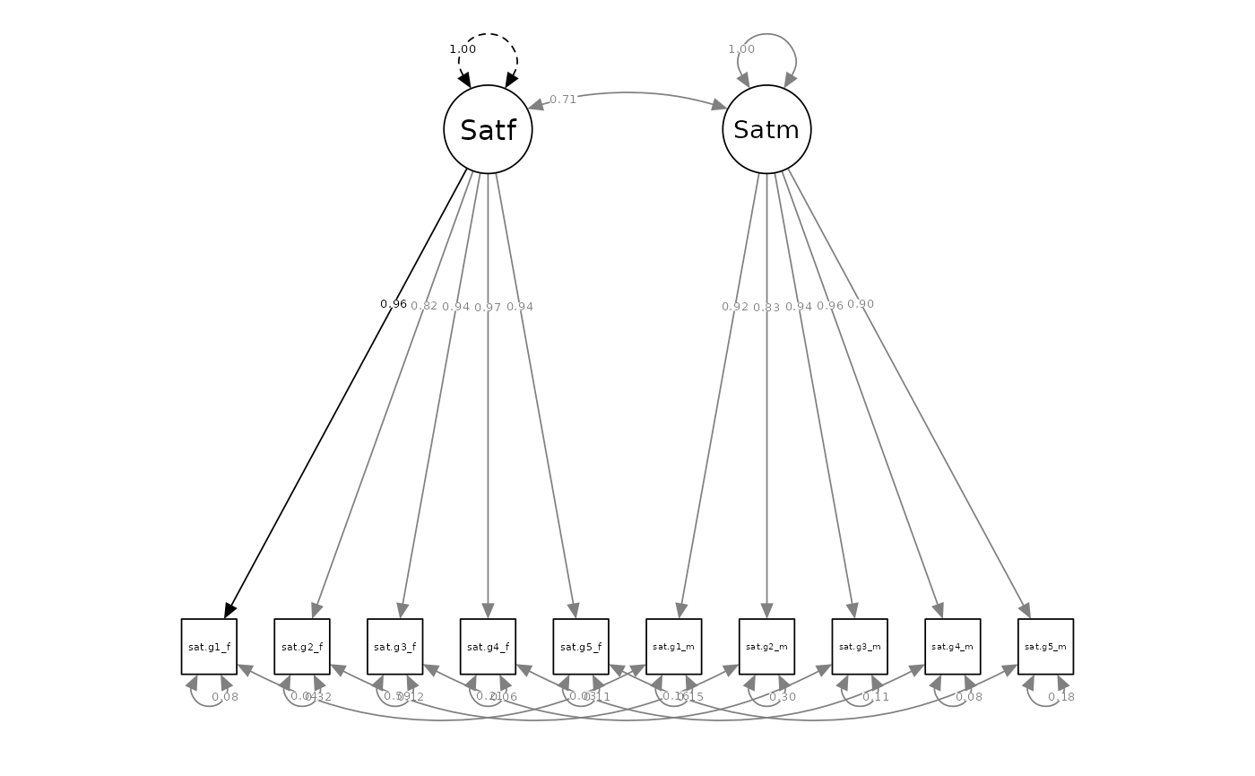

Thus, in little more than a dozen lines of code, researchers can script, fit, compare, and output a series of dyadic invariance comparisons using the Correlated Dyadic Factors Model. From this, researchers would learn that the satisfaction measure demonstrates reasonable configural, loading, and intercept invariance between partners, and that the latent ICC between partner’s satisfaction levels is 0.71, z = 16.15, p <.001 (95% CI: 0.62, 0.8).

5. Consider Optional Indexes and Output

A remaining question would be: if our chosen model fails to demonstrate residual invariance, which indicator(s) are responsible for introducing the noninvariance? The outputConstraintTab() function from dySEM, while not strictly necessary, offers supplemental functionality to help answer this question.

Users simply enter the lavaan model responsible for the statistically significant degradation of model fit, and are provided with a table of each dyadic invariance constraint, by indicator, and its Lagrange multiplier test statistic and corresponding test:


outputConstraintTab(sat.resid.mod) |> 
  gt()

param1	constraint	param2	chi2	df	pvalue	sig
Satf =~ sat.g1_f	==	Satm =~ sat.g1_m	1.131	1	0.288	NA
Satf =~ sat.g2_f	==	Satm =~ sat.g2_m	0.633	1	0.426	NA
Satf =~ sat.g3_f	==	Satm =~ sat.g3_m	0.060	1	0.806	NA
Satf =~ sat.g4_f	==	Satm =~ sat.g4_m	1.839	1	0.175	NA
Satf =~ sat.g5_f	==	Satm =~ sat.g5_m	3.603	1	0.058	NA
sat.g1_f ~1	==	sat.g1_m ~1	0.057	1	0.812	NA
sat.g2_f ~1	==	sat.g2_m ~1	1.316	1	0.251	NA
sat.g3_f ~1	==	sat.g3_m ~1	0.048	1	0.827	NA
sat.g4_f ~1	==	sat.g4_m ~1	0.103	1	0.748	NA
sat.g5_f ~1	==	sat.g5_m ~1	2.090	1	0.148	NA
sat.g1_f ~~ sat.g1_f	==	sat.g1_m ~~ sat.g1_m	22.977	1	0.000	***
sat.g2_f ~~ sat.g2_f	==	sat.g2_m ~~ sat.g2_m	0.263	1	0.608	NA
sat.g3_f ~~ sat.g3_f	==	sat.g3_m ~~ sat.g3_m	0.317	1	0.573	NA
sat.g4_f ~~ sat.g4_f	==	sat.g4_m ~~ sat.g4_m	2.422	1	0.120	NA
sat.g5_f ~~ sat.g5_f	==	sat.g5_m ~~ sat.g5_m	17.185	1	0.000	***

In this particular instance, significant noninvariance was only introduced by forcing the constraint on the residual variances for the 1st and 5th items.