Fitting and Interpreting the Latent Actor-Partner Interdependence Model (L-APIM) • dySEM

Fair Use of this Tutorial

This tutorial is a supplemental material from the following article:

Sakaluk, J. K., & Camanto, O. J. (2025). Dyadic Data Analysis via Structural Equation Modeling with Latent Variables: A Tutorial with the dySEM package for R.

This article is intended to serve as the primary citation of record for the dySEM package’s functionality for the techniques described in this tutorial. If this tutorial has informed your modeling strategy (including but not limited to your use of dySEM), please cite this article.

The citation of research software aiding in analyses—like the use of dySEM—is a required practice, according to the Journal Article Reporting Standards (JARS) for Quantitative Research in Psychology (Appelbaum et al., 2018).

Furthermore, citations remain essential for our development team to demonstrate the impact of our work to our local institutions and our funding sources, and with your support, we will be able to continue justifying our time and efforts spent improving dySEM and expanding its reach.

Overview

The L-APIM is a “bi-construct” dyadic SEM (i.e., used to represent dyadic data about two constructs—like latent relationship satisfaction and latent relationship commitment).

It contains:

parallel/identical sets of latent variables, one pair of which are the predictors (e.g., each partner’s latent relationship satisfaction), and the other pair of which are the criterion/outcomes (e.g., each partner’s latent relationship commitment), onto each of which
each partner’s observed variables discriminantly load (i.e., one partner’s observed satisfaction and commitment variables onto their respective satisfaction and commitment factors, and the other partner’s observed variables onto their respective factors)

It also features several varieties of covariances (or correlations, depending on scale-setting/output standardization):

those between the two latent predictor variables, across partners (effectively, a latent “intraclass” correlation coefficient, when standardized; e.g., Partner A’s latent satisfaction with Partner B’s latent satisfaction),
those between the two latent outcome variables, across partners (effectively, latent intraclass residual correlation, when standardized; e.g., the association between what latent substance is left over between Partner A’s latent commitment and Partner B’s latent commitment, after taking each of their latent satisfaction levels into account) and
several between the residual variances of the same observed variables across each partner (e.g., between Item 1 for Partner A and Partner B; another between Item 2 for Partner A and Partner B, etc.,).

Finally, and most distinctively, it also features a few slopes, of different kinds, between the latent variables:

“actor” effects are slopes estimated from each partner’s latent predictor to their own latent outcome (e.g., Partner A’s latent relationship satisfaction predicting their own latent relationship commitment, and Partner B’s latent relationship satisfaction predicting their own latent relationship commitment),
“partner” effects are slopes estimated from each partner’s latent predictor to their partner’s latent outcome (e.g., Partner A’s latent relationship satisfaction predicting Partner B’s latent relationship commitment, and Partner B’s latent relationship satisfaction predicting Partner A’s latent relationship commitment)

These slopes may be estimated separately for each partner (i.e., producing unique actor and partner effect for each partner) to produce a “distinguishable” L-APIM, or some or all of these slopes may be constrained (i.e., producing a shared/pooled effect for a given slope(s)) introduce some level of “indistinguishability” to the structural model. Further, sometimes researchers are interested in estimating a boutique parameter that captures the ratio between actor and partner effects—the k parameter—in order to characterize the “pattern” of dyadic effects.

The observed (i.e., non-latent) APIM is, by an incredibly wide margin, the most popular bi-construct dyadic data model. Though the L-APIM is not as popular (likely owing to its increased programming difficulty—a barrier we hope dySEM helps to remove), it is well-suited to address the problems that measurement error and statistical control interactively introduce that would otherwise contaminate the insights of the observed APIM. It also enables researchers to simultaneously appraise dyadic invariance for both the latent predictors and latent outcomes—a tacit assumption of informative comparisons of actor and partner effects across partners and the estimation of the k parameter.

Packages and Data

This exemplar makes use of the dplyr, janitor, gt, dySEM, and lavaan (Rosseel, 2012) packages, as well as the development version of the dynamic package.

library(dplyr) #for data management
library(janitor) # for cleaning up data frames for tabling
library(gt) #for reproducible tabling
library(dySEM) #for dyadic SEM scripting and outputting
library(lavaan) #for fitting dyadic SEMs

#devtools::install_github("melissagwolf/dynamic")
#library(dynamic) # development version for calculating 3DFIs

For this exemplar, we use the commitmentQ dataset from dySEM, collected using the “global” version of items for relationship satisfaction from the Rusbult et al. (1998) Investment Model Scale. This dataset includes the very same items as the commitmentM data set used in the exemplar for the CDFM, except responses come from 118 LGBTQ+ dyads (distinguished by partner “1” or “2”) and the variable naming elements follow a “spi” pattern. In this bi-construct exemplar, we will make use of both the responses to the satisfaction and commitment items:

com_dat <- commitmentQ

com_dat |> 
  as_tibble() 
#> # A tibble: 118 × 20
#>    sat.g.1_1 sat.g.1_2 sat.g.1_3 sat.g.1_4 sat.g.1_5 com.1_1 com.1_2 com.1_3
#>        <int>     <int>     <int>     <int>     <int>   <int>   <int>   <int>
#>  1         8         8         5         7         8       8       6       7
#>  2         8         8         8         1         8       9       9       1
#>  3         4         6         4         6         4       9       9       9
#>  4         4         4         5         4         5       7       5       7
#>  5         1         1         1         1         1       9       9       1
#>  6         6         8         7         9         5       9       9       1
#>  7         9         9         7         8         8       9       9       1
#>  8         9         9         9         9         9       9       9       9
#>  9         5         6         5         5         6       9       9       1
#> 10         9         9         9         9         9       9       9       1
#> # ℹ 108 more rows
#> # ℹ 12 more variables: com.1_4 <int>, com.1_5 <int>, sat.g.2_1 <int>,
#> #   sat.g.2_2 <int>, sat.g.2_3 <int>, sat.g.2_4 <int>, sat.g.2_5 <int>,
#> #   com.2_1 <int>, com.2_2 <int>, com.2_3 <int>, com.2_4 <int>, com.2_5 <int>

1. Scraping the Variables

We first scrape the satisfaction and commitment indicators with scrapeVarCross(); when two constructs have information for their indicators scraped, researchers can make use of the y_ arguments (e.g., y_order, y_stem) that parallel the x_ arguments for specifying the variable naming pattern that x (satisfaction) and y (commitment) indicators follow (though the function currently presumes that the same distinguishing characters—in this case, “1’ and”2”—are used for both x and y indicators):


apim_dvn <- scrapeVarCross(dat = com_dat, 
                           x_order = "spi", x_stem = "sat.g", x_delim1 = ".",x_delim2="_",  
                           y_order="spi", y_stem="com", y_delim1 = ".", y_delim2="_",
                           distinguish_1="1", distinguish_2="2")

2. Scripting the Model(s)

Scripting L-APIMs is subsequently expeditious with the scriptAPIM() function. All that is required is a “dvn” of scraped information for x- and y- indicators, and (arbitrary) names for the latent X and latent Y variables. Users then can invoke whatever optional argumentation they wish to control dyadic measurement invariance constraints for their x- and/or y-indicators through the constr_dy_x_meas and constr_dy_y_meas arguments. Likewise, structural level equality constraints on features of latent x and latent y (i.e., variances and means) are controlled through constr_dy_x_struct and constr_dy_y_struct, while users control equality constraints on the latent slopes (i.e., actor and/or partner effects) through the constr_dy_xy_struct argument.

In an effort to boost the inclusivity of dyadic data analysis methods (Sakaluk et al., 2025), scriptAPIM() defaults to a fully indistinguishable model—one in which loadings, intercepts, residuals, latent variances, latent means, and latent slopes are all constrained to be equal across dyad members. The burden is thereby placed on researchers to provide evidence for a less parsimonious model (Kenny et al., 2006), by manually specifying less constrained models and testing against the fully indistinguishable model as a baseline. Finally, scriptAPIM() enables researchers to optionally estimate the k parameter (Kenny & Ledermann, 2010) based on the latent slopes, by setting the est_k argument to TRUE; the estimation of k is programmed to automatically adjust depending what constraints, if any, are made on actor and/or partner effects.

Any model generated by scriptAPIM() can be outputted to a .txt file for transparent sharing of research materials, through the use of the optional writeTo and fileName arguments.

Here, we depict the process of fitting competing L-APIMs that have indistinguishable measurement models, latent variances, and means, while indulging different patterns of actor- and partner-effects, and estimating k in each model:


#actor and partner paths constrained by default
apim.script.indist <-  scriptAPIM(apim_dvn, lvxname = "Sat", lvyname = "Com", est_k = TRUE)

#only constrain partner effects
apim.script.free.act <-  scriptAPIM(apim_dvn, lvxname = "Sat", lvyname = "Com", est_k = TRUE, constr_dy_xy_struct = c("partners"))

#only constrain actor effects
apim.script.free.part <-  scriptAPIM(apim_dvn, lvxname = "Sat", lvyname = "Com", est_k = TRUE, constr_dy_xy_struct = c("actors"))

#freely estimate both actor and partner effects
apim.script.free.actpart <-  scriptAPIM(apim_dvn, lvxname = "Sat", lvyname = "Com", est_k = TRUE, constr_dy_xy_struct = c("none"))

3. Fitting the Model(s)

We can then pass these scripted models to lavaan for model fitting:

apim.fit.indist <- cfa(apim.script.indist, data = com_dat)
apim.fit.free.act <- cfa(apim.script.free.act, data = com_dat)
apim.fit.free.part <- cfa(apim.script.free.part, data = com_dat)
apim.fit.free.actpart <- cfa(apim.script.free.actpart, data = com_dat)

4. Outputting and Interpreting the Model(s)

#compare competing models
comp_act <- anova(apim.fit.indist, apim.fit.free.act)
comp_part <- anova(apim.fit.indist, apim.fit.free.part)
comp_actpart <- anova(apim.fit.indist, apim.fit.free.actpart)

#clean up for reporting
comp_act <- janitor::clean_names(comp_act)
comp_part <- janitor::clean_names(comp_part)
comp_actpart <- janitor::clean_names(comp_actpart)

#rounding for reporting
chisq_diff_act <- round(comp_act$chisq_diff, 2)
p_act <- round(comp_act$pr_chisq, 2)

chisq_diff_part <- round(comp_part$chisq_diff, 2)
p_part <- round(comp_part$pr_chisq, 2)

chisq_diff_actpart <- round(comp_actpart$chisq_diff, 2)
p_actpart <- round(comp_actpart$pr_chisq, 2)

mis_actpart <- fitMeasures(apim.fit.free.actpart, c("rmsea", "cfi"))

Interestingly, while neither freely estimating the actor paths, $\chi^2$ (1) = 0.71, p = 0.4, or partner paths, $\chi^2$ (1) = 0.27, p = 0.61, significantly improved the fit of the model, freely estimating both actor and partner paths did, $\chi^2$ (2) = 9.78, p = 0.01. That said, the freely estimated model did not fit the data particularly well according to traditional model fit cutoffs (Hu & Bentler, 1999), with RMSEA = 0.11 and CFI = 0.886.

outputParamFig() makes it easy to visualize the parameter estimates from the L-APIM, via semPlot package (Epskamp, 2015):


outputParamFig(fit = apim.fit.free.actpart, figtype = "unstandardized")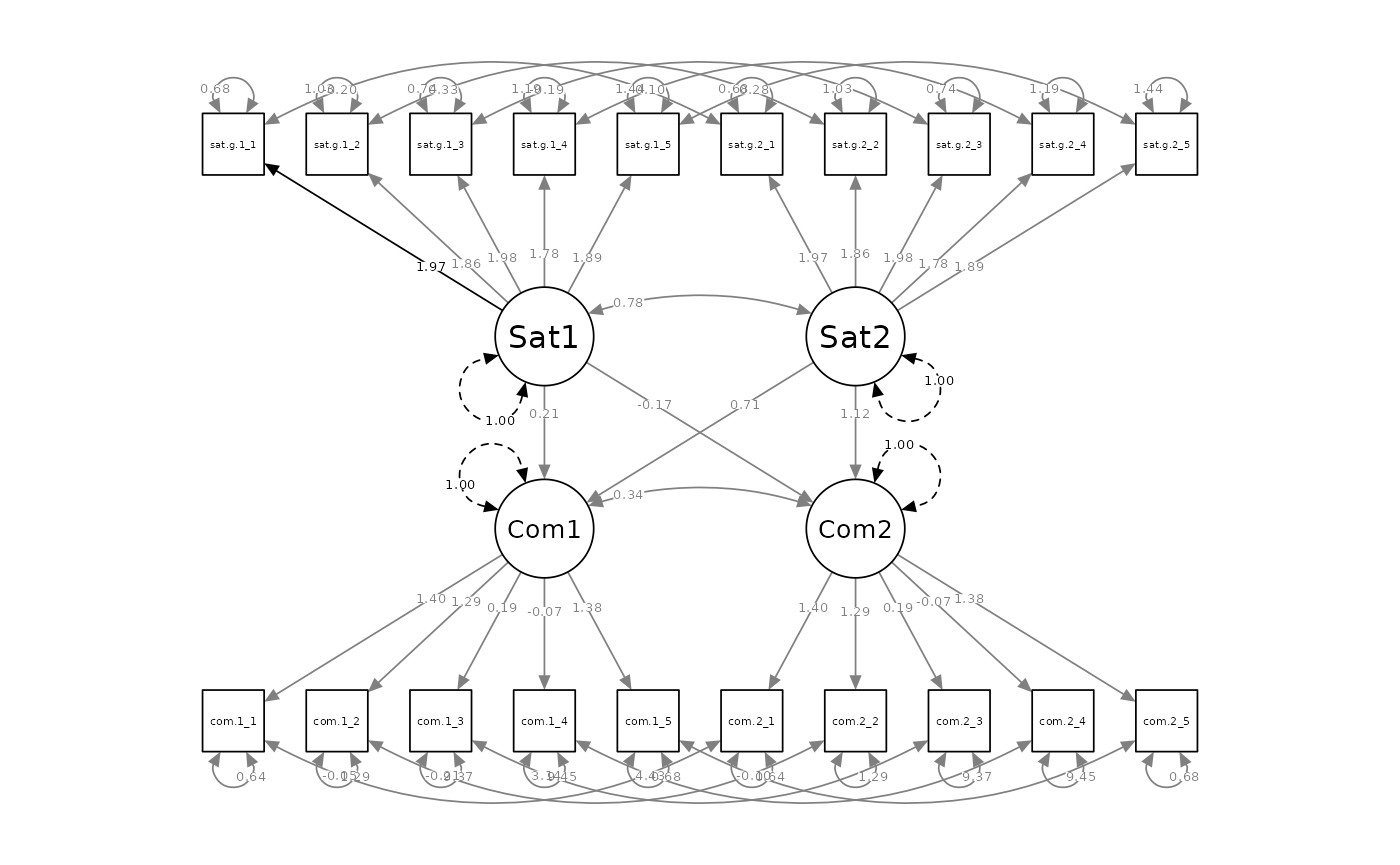

Likewise, outputParamTab() provides reproducible tables of APIM output, and can be directed to provide only structural model output (as we demonstrate), measurement model output, or both:


outputParamTab(apim_dvn, model = "apim", fit = apim.fit.free.actpart, 
               tabletype = "structural") |> 
  gt()

lhs	op	rhs	Label	Estimate	SE	p-value	95%CI LL	95%CI UL	Std. Estimate
Sat1	~~	Sat1	psix	1.000	0.000	NA	1.000	1.000	1.000
Sat2	~~	Sat2	psix	1.000	0.000	NA	1.000	1.000	1.000
Sat1	~~	Sat2		0.776	0.043	< .001	0.691	0.860	0.776
Com1	~~	Com1	psiy	1.000	0.000	NA	1.000	1.000	0.559
Com2	~~	Com2	psiy	1.000	0.000	NA	1.000	1.000	0.503
Com1	~~	Com2		0.335	0.102	0.001	0.135	0.536	0.335
Com1	~	Sat1	a1	0.213	0.180	0.235	-0.139	0.565	0.159
Com2	~	Sat2	a2	1.123	0.210	< .001	0.712	1.534	0.796
Com1	~	Sat2	p1	0.712	0.191	< .001	0.338	1.086	0.533
Com2	~	Sat1	p2	-0.174	0.184	0.345	-0.533	0.186	-0.123
k1	:=	p1/a1	k1	3.342	3.527	0.343	-3.570	10.255	3.342
k2	:=	p2/a2	k2	-0.155	0.143	0.279	-0.434	0.125	-0.155

In this instance, the output suggests that whereas Partner 2’s level of satisfaction is a significant predictor of their own commitment (a2) and their partner’s (p1), Partner 1’s level of satisfaction is not a significant predictor of either partner’s level of commitment. Meanwhile, Partner 1’s k parameter is so imprecise (owing to its modest actor effect) that its confidence interval spans all possible dyadic patterns, while Partner 2’s k parameter is more indicative of an actor-only pattern (0), such that we can reject the possibility of either a contrast-pattern (-1) or a couple-pattern (1).

5. Optional Indexes and Output

This exemplar of the L-APIM also serves to briefly demonstrate the benefits of building dySEM on top of the foundation of lavaan, as any core or external improvement or modernation for lavaan-based functionality can thereby benefit dySEM. McNeish’s work (McNeish et al., 2018), for example, has brought appropriate renewed attention to the limits of depending on the cutoffs for model fit indexes that were popularized, most successfully, by Hu and Bentler (Hu & Bentler, 1999). Subsequently, McNeish and colleagues have provided lavaan-friendly functionality to calculate so-called “dynamic” fit indexes, which identify simulation-generated targets for model fit indexes that are calibrated to a given fitted model (McNeish, 2023; McNeish & Manapat, 2024; McNeish & Wolf, 2022, 2023). More recently, McNeish and Wolf have proposed Direct Discrepancy Dynamic Fit Index (“DD-DFI” or “3DFI”) cutoffs, which are robust in application across many kinds of fitted models, response scales, estimators, and missing data conditions (McNeish & Wolf, 2024). And with their dynamic package for R, it is quite straightforward to use 3DFIs, with dySEM, to perform a more rigorous appraisal of the fit of our selected L-APIMs: a practice that, whenever possible, we recommend as the default approach for the appraisal of dyadic SEMs with dySEM when their features match the requirements of 3DFIs—namely, in the absence of a mean structure.

To evaluate the dynamic fit of our selected L-APIM, we can quickly re-fit it without a mean structure (to make it appropriate for calculating 3DFIs) using the optional includeMeanStruct argument (and setting it to FALSE) for scriptAPIM(), which will ensure no intercepts or latent means are estimated (you can verify this for yourself with summary()):

#without mean structure
#freely estimate both actor and partner effects
apim.script.free.actpart.noms <-  scriptAPIM(apim_dvn, lvxname = "Sat", lvyname = "Com", est_k = TRUE, constr_dy_xy_struct = c("none"), includeMeanStruct = FALSE)

apim.fit.free.actpart.noms <- cfa(apim.script.free.actpart.noms, data = com_dat)

Then, it’s as simple as supplying the fitted lavaan model to the dynamic package’s DDDFI() function. Because this is a simulation-based function, it’s good practice to set a random seed (to ensure you can get the same numeric results from run to run):

set.seed(519)
DDDFI(apim.fit.free.actpart.noms)

Note: since the DDDFI() function is not yet in the CRAN version of dynamic, we can’t reproducibly run it and include the output here, in this automatically compiling online tutorial, but you can run this code in your own R session to see the results.

Based on these 3DFI targets, both our observed model fit values of RMSEA = 0.11 and CFI = 0.886 fall between the “Fair” and “Mediocre” level of fit. This is likely driven (in part) by exceptionally low loading values observed for some of the commitment items (which we would further explore, if this were a real analysis and we were so inclined).