Fitting and Interpreting the Multiple Correlated Dyadic Factors Model (M-CDFM)

Fair Use of this Tutorial

This tutorial is a supplemental material from the following article:

Prine-Munroe, M., Sakaluk, J. K., Camanto, O., & Quinn-Nilas, C. (2025). Evaluating Multi-Factor Dyadic Invariance in Couples’ Relationship Satisfaction Using dySEM.

This article is intended to serve as the primary citation of record for the dySEM package’s functionality for fitting and interpreting the the Multiple Correlated Dyadic Factors Model with the help of the scriptMultiCor()/scriptCFA() function (and others) in dySEM. If this tutorial has informed your modeling strategy (including but not limited to your use of dySEM), please cite this article.

The citation of research software aiding in analyses—like the use of dySEM—is a required practice, according to the Journal Article Reporting Standards (JARS) for Quantitative Research in Psychology (Appelbaum et al., 2018).

Furthermore, citations remain essential for our development team to demonstrate the impact of our work to our local institutions and our funding sources, and with your support, we will be able to continue justifying our time and efforts spent improving dySEM and expanding its reach.

Overview

The M-CDFM is a “multi-construct” dyadic SEM (i.e., used to represent dyadic data about more than two constructs—like different features of relationship quality, e.g., Fletcher et al., 2000).

It contains:

parallel/identical sets of latent variables, onto which
each partner’s observed variables discriminantly load (i.e., one partner’s observed variables onto their respective factors, and the other partner’s observed variables onto their respective factors)

It also features several varieties of covariances (or correlations, depending on scale-setting/output standardization):

those between two latent variables for the same construct across partners (effectively, latent “intraclass” correlation coefficients, when standardized; e.g., Partner A’s latent commitment with Partner B’s latent commitment),
those between two latent variables for different constructs within each partner (e.g., effectively, latent “intrapartner” correlation coefficients, when standardized; e.g., Partner A’s latent commitment with Partner A’s latent passion),
those between two latent variables for different constructs across partners (e.g., effectively, latent “interpartner” correlation coefficients, when standardized; e.g., Partner A’s latent commitment with Partner B’s latent passion) , and
several between the residual variances of the same observed variables across each partner (e.g., between Item 1 for Partner A and Partner B; another between Item 2 for Partner A and Partner B, etc.,).

The M-CDFM is typically the model people mean when they refer to “dyadic CFA”, though dyadic CFA is more of a statistical framework that could be used to fit multi-construct dyadic data that corresponds to other data generating mechanisms of uni-construct dyadic data (e.g., from multiple constructs embodying Univariate Dyadic Factor Models). It is therefore likely the most common model used for psychometric tests of dyadic data.

Packages and Data

This exemplar makes use of the dplyr, gt, dySEM, and lavaan (Rosseel, 2012) packages.


library(dplyr) #for data management
library(gt) #for reproducible tabling
library(dySEM) #for dyadic SEM scripting and outputting
library(lavaan) #for fitting dyadic SEMs

For this exemplar, we use two built-in datasets from dySEM (focusing more on one). Of primary interest, the pnrqM dataset corresponds to data from a short-form of the Positive-Negative Relationship Quality Scale (PNRQ; Rogge et al., 2017) from 219 (M)ixed-sex couples (including 4 items each for positive and negative). More information about this data set can be found in Prine et al. (under review).

All variables in this data frame follow a “sip” naming pattern, with a delimiting “_” between the item number and distinguishing partner character:


pnrqM_dat <- pnrqM

pnrqM_dat |> 
  as_tibble()
#> # A tibble: 219 × 16
#>    sat.pnrq1_w sat.pnrq2_w sat.pnrq3_w sat.pnrq4_w dsat.pnrq1_w dsat.pnrq2_w
#>          <dbl>       <dbl>       <dbl>       <dbl>        <dbl>        <dbl>
#>  1           5           5           5           5            1            1
#>  2           6           6           6           6            1            1
#>  3           5           5           4           6            3            5
#>  4           5           5           6           5            1            2
#>  5           4           4           5           4            1            1
#>  6           4           4           4           3            1            1
#>  7           5           5           5           5            1            1
#>  8           5           5           5           5            1            1
#>  9           5           6           6           6            1            1
#> 10           3           3           4           4            1            1
#> # ℹ 209 more rows
#> # ℹ 10 more variables: dsat.pnrq3_w <dbl>, dsat.pnrq4_w <dbl>,
#> #   sat.pnrq1_m <dbl>, sat.pnrq2_m <dbl>, sat.pnrq3_m <dbl>, sat.pnrq4_m <dbl>,
#> #   dsat.pnrq1_m <dbl>, dsat.pnrq2_m <dbl>, dsat.pnrq3_m <dbl>,
#> #   dsat.pnrq4_m <dbl>

We will also use data from the prqcQ dataset, which contains data from 118 queer couples responding to the Perceived Relationship Quality Components Inventory (Fletcher et al., 2000) (including 3 items each for satisfaction, commitment, intimacy, trust, passion, and love). While substantive analyses of this data set have not yet been reported, the data collection took place in parallel to the analyses reported in Sakaluk et al. (2021).

In contrast to pnrqM, variable names in the prqcQ data frame follow the “spi” naming pattern:


prqc_dat <- prqcQ

prqc_dat |> 
  as_tibble()
#> # A tibble: 118 × 36
#>    prqc.1_1 prqc.1_2 prqc.1_3 prqc.1_4 prqc.1_5 prqc.1_6 prqc.1_7 prqc.1_8
#>       <int>    <int>    <int>    <int>    <int>    <int>    <int>    <int>
#>  1        5        6        5        5        4        6        6        6
#>  2        7        7        7        7        7        7        7        7
#>  3        4        3        4        7        7        7        1        2
#>  4        5        5        7        6        5        7        5        7
#>  5        7        7        7        7        7        7        7        7
#>  6        5        5        5        6        7        7        6        6
#>  7        7        7        7        7        6        6        6        7
#>  8        7        7        7        7        7        7        7        7
#>  9        4        4        4        6        6        6        4        6
#> 10        7        7        7        7        7        7        7        7
#> # ℹ 108 more rows
#> # ℹ 28 more variables: prqc.1_9 <int>, prqc.1_10 <int>, prqc.1_11 <int>,
#> #   prqc.1_12 <int>, prqc.1_13 <int>, prqc.1_14 <int>, prqc.1_15 <int>,
#> #   prqc.1_16 <int>, prqc.1_17 <int>, prqc.1_18 <int>, prqc.2_1 <int>,
#> #   prqc.2_2 <int>, prqc.2_3 <int>, prqc.2_4 <int>, prqc.2_5 <int>,
#> #   prqc.2_6 <int>, prqc.2_7 <int>, prqc.2_8 <int>, prqc.2_9 <int>,
#> #   prqc.2_10 <int>, prqc.2_11 <int>, prqc.2_12 <int>, prqc.2_13 <int>, …

1. Scraping the Variables

Users will take note that the pnrqM dataset contains variables for items for which there are distinctive stems for the positive and negative subscales (i.e., “sat.pnrq”, “dsat.pnrq”), whereas the prqcQ dataset contains a repetitive uninformative stem (“prqc”), despite the presence of multidimensionality. Rest assured, scrapeVarCross() has been developed with functionality to scrape variable information from both kinds of stems from multidimensional instruments. Further, scraping variable information remains relatively straightforward (and the key to unlocking the powerful functionality of dySEM‘s scripters), with just one added “twist” from the simpler case of uni-construct or bi-construct models: the creation of a named list spelling out the naming ’formula’ for each set of indicators.

Distinctive Indicator Stems (with `pnrqM`)

The case when indicators have distinctive stems—usually indicating the putative factor onto which they load (e.g., “sat”, “com”)—is the most straightforward to scrape with scrapeVarCross().

In this case, users will need to provide the names of the latent variables, the stem for each set of indicators, and the delimiters used in the variable names. In the case of the pnrqM exemplar (i.e., when stems are distinct), the named list must contain the following four elements/vectors (and the names of these elements/vectors must follow what is shown below):

lvnames: a vector of the (arbitrary) names that will be used for the latent variables in the lavaan script
stem: a vector containing each distinctive stem for each set of indicators (in this case: “sat” and “dsat”)— scrapeVarCross() will use these to search for indicators with matching stems
delim1: a vector containing the first delimiter used in the variable names (e.g., “.”, “_“)— scrapeVarCross() will use these to search for indicators with matching patterns of delimination
delim2: a vector containing the second delimiter used in the variable names— scrapeVarCross() will use these to search for indicators with matching patterns of delimination

Each of these elements/vectors must be of the same length, and the order of the elements in each vector must correspond to the order of the latent variables in lvnames. And so, saving this named list (in essence, the “recipe card” of indicator names for each factor) into its own object:


#When different factor use distinct stems:
pnrqMList <- list(lvnames = c("Sat", "Dsat"),
stem = c("sat.pnrq", "dsat.pnrq"),
delim1 = c("", ""),#no delimeter between stem and item number
delim2 = c("_", "_"))

This list can then be passed to scrapeVarCross() to scrape the variable names from the pnrqM data frame, using the var_list argument. The var_list_order argument must then be set to indicate that the variables follow the “sip” naming pattern, and distinguishing characters must also be specified with the distinguish_1 and distinguish_2 arguments¹:


dvnPNRQ <- scrapeVarCross(pnrqM,
var_list = pnrqMList,
var_list_order = "sip",
distinguish_1 = "w",
distinguish_2 = "m")
#> 
#> ── Variable Scraping Summary ──
#> 
#> ✔ Successfully scraped 2 latent variables
#> ℹ Sat: 4 indicators for P1 (w), 4 indicators for P2 (m)
#> ℹ Dsat: 4 indicators for P1 (w), 4 indicators for P2 (m)
#> ℹ Total indicators: 16

The resulting dvn remains as unremarkable as ever, but continues to serve as the foundation for unlocking the functionality of multi-construct scripters in dySEM. The only difference from the one-construct use-case of scrapeVarCross() is that the $p1xvarnames and $p2xvarnames elements now contain a nested set of vectors of variable names (as opposed to only set of variable names):


dvnPNRQ
#> $p1xvarnames
#> $p1xvarnames$Sat
#> [1] "sat.pnrq1_w" "sat.pnrq2_w" "sat.pnrq3_w" "sat.pnrq4_w"
#> 
#> $p1xvarnames$Dsat
#> [1] "dsat.pnrq1_w" "dsat.pnrq2_w" "dsat.pnrq3_w" "dsat.pnrq4_w"
#> 
#> 
#> $p2xvarnames
#> $p2xvarnames$Sat
#> [1] "sat.pnrq1_m" "sat.pnrq2_m" "sat.pnrq3_m" "sat.pnrq4_m"
#> 
#> $p2xvarnames$Dsat
#> [1] "dsat.pnrq1_m" "dsat.pnrq2_m" "dsat.pnrq3_m" "dsat.pnrq4_m"
#> 
#> 
#> $xindper
#> [1] 8
#> 
#> $dist1
#> [1] "w"
#> 
#> $dist2
#> [1] "m"
#> 
#> $indnum
#> [1] 16

Non-Distinctive Indicator Stems (with `prqcQ`)

The case when indicators have non-distinctive stems only requires that your named list—that you later supply to scrapeVarCross()—has two more elements/vectors. Currently, this functionality assumes indicators from the same latent variable (e.g., items measuring Satisfaction) are clustered together, sequentially, in item number (e.g., prqc.1_1 prqc.1_2 prqc.1_3) rather than being interspersed with items from other latent variables (e.g., prqc.1_1 prqc.1_5, prqc.1_8).

The additional arguments that must be added to the named list are:

min_num: a vector containing the item number in the sequence of non-distinctively named indicators that corresponds to the first item for each latent variable (e.g., 1, 4, 7, 10, 13, 16 for Satisfaction, Commitment, Intimacy, Trust, Passion, and Love, respectively), and
max_num: a vector containing the item number in the sequence of non-distinctively named indicators that corresponds to the last item for each latent variable (e.g., 3, 6, 9, 12, 15, 18 for Satisfaction, Commitment, Intimacy, Trust, Passion, and Love, respectively).


#When different factor use non-distinct stems:
prqcList <- list(lvnames = c("Sat", "Comm", "Intim", "Trust", "Pass", "Love"),
stem = c("prqc", "prqc", "prqc", "prqc", "prqc", "prqc"),
delim1 = c(".", ".", ".", ".", ".", "."),
delim2 = c("_", "_", "_", "_", "_", "_"),
min_num = c(1, 4, 7, 10, 13, 16),
max_num = c(3, 6, 9, 12, 15, 18))

This named list can then be passed to scrapeVarCross() to the same effect (noting that in this case, the prqcQ data set follows a “spi” naming pattern, and “1” and “2” as the distinguishing characters):


dvnPRQC<- scrapeVarCross(prqcQ,
var_list = prqcList,
var_list_order = "spi",
distinguish_1 = "1",
distinguish_2 = "2")
#> 
#> ── Variable Scraping Summary ──
#> 
#> ✔ Successfully scraped 6 latent variables
#> ℹ Sat: 3 indicators for P1 (1), 3 indicators for P2 (2)
#> ℹ Comm: 3 indicators for P1 (1), 3 indicators for P2 (2)
#> ℹ Intim: 3 indicators for P1 (1), 3 indicators for P2 (2)
#> ℹ Trust: 3 indicators for P1 (1), 3 indicators for P2 (2)
#> ℹ Pass: 3 indicators for P1 (1), 3 indicators for P2 (2)
#> ℹ Love: 3 indicators for P1 (1), 3 indicators for P2 (2)
#> ℹ Total indicators: 36

dvnPRQC
#> $p1xvarnames
#> $p1xvarnames$Sat
#> [1] "prqc.1_1" "prqc.1_2" "prqc.1_3"
#> 
#> $p1xvarnames$Comm
#> [1] "prqc.1_4" "prqc.1_5" "prqc.1_6"
#> 
#> $p1xvarnames$Intim
#> [1] "prqc.1_7" "prqc.1_8" "prqc.1_9"
#> 
#> $p1xvarnames$Trust
#> [1] "prqc.1_10" "prqc.1_11" "prqc.1_12"
#> 
#> $p1xvarnames$Pass
#> [1] "prqc.1_13" "prqc.1_14" "prqc.1_15"
#> 
#> $p1xvarnames$Love
#> [1] "prqc.1_16" "prqc.1_17" "prqc.1_18"
#> 
#> 
#> $p2xvarnames
#> $p2xvarnames$Sat
#> [1] "prqc.2_1" "prqc.2_2" "prqc.2_3"
#> 
#> $p2xvarnames$Comm
#> [1] "prqc.2_4" "prqc.2_5" "prqc.2_6"
#> 
#> $p2xvarnames$Intim
#> [1] "prqc.2_7" "prqc.2_8" "prqc.2_9"
#> 
#> $p2xvarnames$Trust
#> [1] "prqc.2_10" "prqc.2_11" "prqc.2_12"
#> 
#> $p2xvarnames$Pass
#> [1] "prqc.2_13" "prqc.2_14" "prqc.2_15"
#> 
#> $p2xvarnames$Love
#> [1] "prqc.2_16" "prqc.2_17" "prqc.2_18"
#> 
#> 
#> $xindper
#> [1] 18
#> 
#> $dist1
#> [1] "1"
#> 
#> $dist2
#> [1] "2"
#> 
#> $indnum
#> [1] 36

Whether your dvn contains variable information for indicators with distinctive or non-distinctive stems makes no difference to the functionality you can draw upon from dySEM, or how you pass this information to scripters—it remains the same (and straightforward) for both kinds of indicators.

2. Scripting the Model(s)

Continuing with the pnrqM exemplar for this rest of this vignette, we can now quickly script a series of M-CDFMs using the scriptCFA() function (so named given that most imagine a M-CDFM model when conducting “dyadic CFA”), and incrementally layer on more dyadic invariance constraints via the constr_dy_meas argument.

The writeTo and fileName arguments (not depicted here) remain available to those wanting to export a .txt file of their concatenated lavaan script(s) (e.g., for posting on the OSF). scaleset remains fixed-factor, by default, but this is changeable to marker-variable (“MV”) for those interested. Given the consequential nature of this choice (e.g., for interpreting the scale of parameter estimates), we strongly recommend making this argument explicit (despite its implicit default to “FF”):


script.pnrq.config <-  scriptCFA(dvnPNRQ, scaleset = "FF", constr_dy_meas = "none", constr_dy_struct = "none")

script.pnrq.load <-  scriptCFA(dvnPNRQ, scaleset = "FF", constr_dy_meas = c("loadings"), constr_dy_struct = "none")

script.pnrq.int <-  scriptCFA(dvnPNRQ, scaleset = "FF", constr_dy_meas = c("loadings", "intercepts"),constr_dy_struct = "none")

script.pnrq.res <-  scriptCFA(dvnPNRQ, scaleset = "FF",constr_dy_meas = c("loadings", "intercepts", "residuals"), constr_dy_struct = "none")

You can concatenate these scripts, if you wish, using the base cat() function, to make them more human-readable in your console, but beware: the amount of lavaan scripting is considerable (and therefore we do not show what it returns here):


cat(script.pnrq.config)

3. Fitting the Model(s)

All of these models can now be fit with whichever lavaan wrapper the user prefers, and with their chosen analytic options (e.g., estimator, missing data treatment, etc.); our demonstration uses default specifications for cfa():


pnrq.config.mod <- cfa(script.pnrq.config, data = pnrqM_dat)

pnrq.load.mod <- cfa(script.pnrq.load, data = pnrqM_dat)

pnrq.int.mod <- cfa(script.pnrq.int, data = pnrqM_dat)

pnrq.res.mod <- cfa(script.pnrq.res, data = pnrqM_dat)

4. Outputting and Interpreting the Model(s)

As with the CDFM, competing nested M-CDFMs—like for dyadic invariance testing with a larger measure—can be compared with the base anova() function:


anova(pnrq.config.mod, pnrq.load.mod, pnrq.int.mod, pnrq.res.mod)
#> 
#> Chi-Squared Difference Test
#> 
#>                  Df    AIC    BIC  Chisq Chisq diff   RMSEA Df diff Pr(>Chisq)
#> pnrq.config.mod  90 5777.9 5985.4 371.34                                      
#> pnrq.load.mod    96 5788.8 5976.2 394.24     22.904 0.11582       6  0.0008294
#> pnrq.int.mod    102 5781.1 5948.5 398.57      4.325 0.00000       6  0.6327806
#> pnrq.res.mod    110 5816.9 5957.4 450.33     51.759 0.16139       8  1.874e-08
#>                    
#> pnrq.config.mod    
#> pnrq.load.mod   ***
#> pnrq.int.mod       
#> pnrq.res.mod    ***
#> ---
#> Signif. codes:  0 '***' 0.001 '**' 0.01 '*' 0.05 '.' 0.1 ' ' 1

Or, for a more reproducible-reporting-friendly option, dySEM’s outputInvarCompTab() function is available, and amenable to other tabling packages/functions (e.g., gt::gt(), as we demonstrate below), and/or can write an .rtf if the user makes use of the writeTo and fileName arguments:


mods <- list(pnrq.config.mod, pnrq.load.mod, pnrq.int.mod, pnrq.res.mod)

outputInvarCompTab(mods) |> 
  gt()

mod	chisq	df	aic	bic	rmsea	cfi	chisq_diff	df_diff	p_diff	aic_diff	bic_diff	rmsea_diff	cfi_diff
configural	371.338	90	5777.881	5985.401	0.122	0.942	NA	NA	NA	NA	NA	NA	NA
loading	394.241	96	5788.784	5976.222	0.122	0.939	22.904	6	0.001	10.904	-9.179	0.000	-0.003
intercept	398.566	102	5781.109	5948.465	0.118	0.939	4.325	6	0.633	-7.675	-27.758	-0.004	0.000
residual	450.325	110	5816.868	5957.447	0.121	0.930	51.759	8	0.000	35.759	8.982	0.004	-0.009

Were one strictly to follow only the likelihood ratio test statistic as a guide, they would reject the possibility of the relatively low bar of loading invariance for the PNRQ, $\chi^2$ (6) = 22.9, p <.001. Of course, other methods of model comparison and selection (and their respective thresholds) are available, and whatever method is chosen probably ought to be preregistered.

Meanwhile, the standard outputters from dySEM are available to help researchers either table and/or visualize their results. Given the complexity of the M-CDFM (often many more factors and items) than the CDFM, we recommend tabling (vs. visualizing) model output:


outputParamTab(dvn = dvnPNRQ, model = "cfa", fit = pnrq.config.mod,
               tabletype = "measurement") |> 
  gt()

Latent Factor	Indicator	Loading	SE	Z	p-value	Std. Loading	Intercept
Sat1	sat.pnrq1_w	1.333	0.069	19.304	< .001	0.971	4.619
Sat1	sat.pnrq2_w	1.353	0.070	19.347	< .001	0.972	4.667
Sat1	sat.pnrq3_w	1.308	0.075	17.520	< .001	0.920	4.814
Sat1	sat.pnrq4_w	1.338	0.076	17.530	< .001	0.920	4.571
Dsat1	dsat.pnrq1_w	0.749	0.048	15.608	< .001	0.858	1.367
Dsat1	dsat.pnrq2_w	0.688	0.048	14.226	< .001	0.811	1.310
Dsat1	dsat.pnrq3_w	1.002	0.053	19.009	< .001	0.964	1.490
Dsat1	dsat.pnrq4_w	0.997	0.053	18.845	< .001	0.961	1.443
Sat2	sat.pnrq1_m	1.202	0.065	18.374	< .001	0.947	4.667
Sat2	sat.pnrq2_m	1.212	0.064	18.866	< .001	0.961	4.743
Sat2	sat.pnrq3_m	1.146	0.068	16.739	< .001	0.897	4.886
Sat2	sat.pnrq4_m	1.233	0.073	16.832	< .001	0.899	4.676
Dsat2	dsat.pnrq1_m	0.803	0.045	17.945	< .001	0.933	1.357
Dsat2	dsat.pnrq2_m	0.776	0.043	18.267	< .001	0.944	1.286
Dsat2	dsat.pnrq3_m	0.933	0.051	18.435	< .001	0.948	1.400
Dsat2	dsat.pnrq4_m	0.872	0.050	17.447	< .001	0.920	1.395

We have also provided a tabletype = "correlation" option to assist with providing reproducible correlation tables for reporting on the intraclass, intrapartner, and interpartner correlations, from larger multi-construct models:


outputParamTab(dvn = dvnPNRQ, model = "cfa", fit = pnrq.config.mod,
               tabletype = "correlation") |> 
  gt()

	Sat1	Dsat1	Sat2	Dsat2
Sat1	—	—	—	—
Dsat1	-0.666***	—	—	—
Sat2	0.829***	-0.515***	—	—
Dsat2	-0.473***	0.642***	-0.504***	—

5. Optional Indexes and Output

Finally, like with the CDFM, users can use additional dySEM functions to output additional information about their model, such as the computation of Lagrange multiplier tests to identify for which items and measurement model parameters there is significant noninvariance:


outputConstraintTab(pnrq.load.mod) |> 
  gt()

param1	constraint	param2	chi2	df	pvalue	sig
Sat1 =~ sat.pnrq1_w	==	Sat2 =~ sat.pnrq1_m	0.021	1	0.885	NA
Sat1 =~ sat.pnrq2_w	==	Sat2 =~ sat.pnrq2_m	0.028	1	0.867	NA
Sat1 =~ sat.pnrq3_w	==	Sat2 =~ sat.pnrq3_m	0.476	1	0.490	NA
Sat1 =~ sat.pnrq4_w	==	Sat2 =~ sat.pnrq4_m	0.504	1	0.478	NA
Dsat1 =~ dsat.pnrq1_w	==	Dsat2 =~ dsat.pnrq1_m	6.039	1	0.014	*
Dsat1 =~ dsat.pnrq2_w	==	Dsat2 =~ dsat.pnrq2_m	9.322	1	0.002	**
Dsat1 =~ dsat.pnrq3_w	==	Dsat2 =~ dsat.pnrq3_m	1.701	1	0.192	NA
Dsat1 =~ dsat.pnrq4_w	==	Dsat2 =~ dsat.pnrq4_m	8.564	1	0.003	**

In this particular example, significant noninvariance is present for the loadings of most of the negative items (all but the third).

If we to compute effect sizes to quantify the magnitude of noninvariance in the PNRQ, we need to generate a “partial invariance” model, in which noninvariant measurement parameters are free to vary between partners, while others remain constrained. For these effect sizes to be accurate, it is crucial that the model contains one or more “anchor items”–items that are free of noninvariance.

To begin this process, we will use outputConstraintTab() to identify which loadings and intercepts are noninvariant:


outputConstraintTab(pnrq.int.mod) |> 
  gt()

param1	constraint	param2	chi2	df	pvalue	sig
Sat1 =~ sat.pnrq1_w	==	Sat2 =~ sat.pnrq1_m	0.013	1	0.909	NA
Sat1 =~ sat.pnrq2_w	==	Sat2 =~ sat.pnrq2_m	0.026	1	0.873	NA
Sat1 =~ sat.pnrq3_w	==	Sat2 =~ sat.pnrq3_m	0.472	1	0.492	NA
Sat1 =~ sat.pnrq4_w	==	Sat2 =~ sat.pnrq4_m	0.540	1	0.462	NA
Dsat1 =~ dsat.pnrq1_w	==	Dsat2 =~ dsat.pnrq1_m	5.840	1	0.016	*
Dsat1 =~ dsat.pnrq2_w	==	Dsat2 =~ dsat.pnrq2_m	9.218	1	0.002	**
Dsat1 =~ dsat.pnrq3_w	==	Dsat2 =~ dsat.pnrq3_m	1.540	1	0.215	NA
Dsat1 =~ dsat.pnrq4_w	==	Dsat2 =~ dsat.pnrq4_m	8.679	1	0.003	**
sat.pnrq1_w ~1	==	sat.pnrq1_m ~1	0.638	1	0.425	NA
sat.pnrq2_w ~1	==	sat.pnrq2_m ~1	0.023	1	0.878	NA
sat.pnrq3_w ~1	==	sat.pnrq3_m ~1	0.003	1	0.959	NA
sat.pnrq4_w ~1	==	sat.pnrq4_m ~1	0.540	1	0.462	NA
dsat.pnrq1_w ~1	==	dsat.pnrq1_m ~1	1.624	1	0.203	NA
dsat.pnrq2_w ~1	==	dsat.pnrq2_m ~1	0.396	1	0.529	NA
dsat.pnrq3_w ~1	==	dsat.pnrq3_m ~1	2.867	1	0.090	NA
dsat.pnrq4_w ~1	==	dsat.pnrq4_m ~1	0.134	1	0.714	NA

This output corroborates what we saw before: there isn’t intercept noninvariance to worry about (though now we have the added peace of mind that this is true for each intercept, individually, not just as a “family” of parameters).

While dySEM does not yet automate the production of partial-invariance model syntax, we can use the model syntax from the intercept invariance model and make some light adjustments:


cat(script.pnrq.int)
#> #Measurement Model
#> 
#> #Loadings
#> Sat1 =~ NA*sat.pnrq1_w + lx1*sat.pnrq1_w + lx2*sat.pnrq2_w + lx3*sat.pnrq3_w + lx4*sat.pnrq4_w
#> Dsat1 =~ NA*dsat.pnrq1_w + lx5*dsat.pnrq1_w + lx6*dsat.pnrq2_w + lx7*dsat.pnrq3_w + lx8*dsat.pnrq4_w
#> Sat2 =~ NA*sat.pnrq1_m + lx1*sat.pnrq1_m + lx2*sat.pnrq2_m + lx3*sat.pnrq3_m + lx4*sat.pnrq4_m
#> Dsat2 =~ NA*dsat.pnrq1_m + lx5*dsat.pnrq1_m + lx6*dsat.pnrq2_m + lx7*dsat.pnrq3_m + lx8*dsat.pnrq4_m
#> 
#> #Intercepts
#> sat.pnrq1_w ~ t1*1
#> sat.pnrq2_w ~ t2*1
#> sat.pnrq3_w ~ t3*1
#> sat.pnrq4_w ~ t4*1
#> dsat.pnrq1_w ~ t5*1
#> dsat.pnrq2_w ~ t6*1
#> dsat.pnrq3_w ~ t7*1
#> dsat.pnrq4_w ~ t8*1
#> 
#> sat.pnrq1_m ~ t1*1
#> sat.pnrq2_m ~ t2*1
#> sat.pnrq3_m ~ t3*1
#> sat.pnrq4_m ~ t4*1
#> dsat.pnrq1_m ~ t5*1
#> dsat.pnrq2_m ~ t6*1
#> dsat.pnrq3_m ~ t7*1
#> dsat.pnrq4_m ~ t8*1
#> 
#> #Residual Variances
#> sat.pnrq1_w ~~ th1*sat.pnrq1_w
#> sat.pnrq2_w ~~ th2*sat.pnrq2_w
#> sat.pnrq3_w ~~ th3*sat.pnrq3_w
#> sat.pnrq4_w ~~ th4*sat.pnrq4_w
#> dsat.pnrq1_w ~~ th5*dsat.pnrq1_w
#> dsat.pnrq2_w ~~ th6*dsat.pnrq2_w
#> dsat.pnrq3_w ~~ th7*dsat.pnrq3_w
#> dsat.pnrq4_w ~~ th8*dsat.pnrq4_w
#> 
#> sat.pnrq1_m ~~ th9*sat.pnrq1_m
#> sat.pnrq2_m ~~ th10*sat.pnrq2_m
#> sat.pnrq3_m ~~ th11*sat.pnrq3_m
#> sat.pnrq4_m ~~ th12*sat.pnrq4_m
#> dsat.pnrq1_m ~~ th13*dsat.pnrq1_m
#> dsat.pnrq2_m ~~ th14*dsat.pnrq2_m
#> dsat.pnrq3_m ~~ th15*dsat.pnrq3_m
#> dsat.pnrq4_m ~~ th16*dsat.pnrq4_m
#> 
#> #Residual Covariances
#> sat.pnrq1_w ~~ sat.pnrq1_m
#> sat.pnrq2_w ~~ sat.pnrq2_m
#> sat.pnrq3_w ~~ sat.pnrq3_m
#> sat.pnrq4_w ~~ sat.pnrq4_m
#> dsat.pnrq1_w ~~ dsat.pnrq1_m
#> dsat.pnrq2_w ~~ dsat.pnrq2_m
#> dsat.pnrq3_w ~~ dsat.pnrq3_m
#> dsat.pnrq4_w ~~ dsat.pnrq4_m
#> 
#> #Structural Model
#> 
#> #Latent (Co)Variances
#> Sat1 ~~ psv1*Sat1 + 1*Sat1
#> Dsat1 ~~ psv2*Dsat1 + 1*Dsat1
#> Sat2 ~~ psv3*Sat2 + NA*Sat2
#> Dsat2 ~~ psv4*Dsat2 + NA*Dsat2
#> Sat1 ~~ psi12*Dsat1
#> Sat1 ~~ psi13*Sat2
#> Sat1 ~~ psi14*Dsat2
#> Dsat1 ~~ psi23*Sat2
#> Dsat1 ~~ psi24*Dsat2
#> Sat2 ~~ psi34*Dsat2
#> 
#> #Latent Means
#> Sat1 ~ a1*1 + 0*1
#> Dsat1 ~ a2*1 + 0*1
#> Sat2 ~ a3*1
#> Dsat2 ~ a4*1

The output of outputConstraintTab() indicated that the loadings for items 1, 2, and 4 of the negative subscale were noninvariant, so we simply “free” these loadings by removing the equality constraints (i.e., the shared parameter labels) for them:


script.pnrq.partial <- '
#Measurement Model

#Loadings (remove l5*, l6*, and l8* for partial invariance
# in Dsat1 and Dsat2)
Sat1 =~ NA*sat.pnrq1_w + lx1*sat.pnrq1_w + lx2*sat.pnrq2_w + lx3*sat.pnrq3_w + lx4*sat.pnrq4_w
Dsat1 =~ NA*dsat.pnrq1_w + dsat.pnrq1_w + dsat.pnrq2_w + lx7*dsat.pnrq3_w + dsat.pnrq4_w
Sat2 =~ NA*sat.pnrq1_m + lx1*sat.pnrq1_m + lx2*sat.pnrq2_m + lx3*sat.pnrq3_m + lx4*sat.pnrq4_m
Dsat2 =~ NA*dsat.pnrq1_m + dsat.pnrq1_m + dsat.pnrq2_m + lx7*dsat.pnrq3_m + dsat.pnrq4_m

#Intercepts
sat.pnrq1_w ~ t1*1
sat.pnrq2_w ~ t2*1
sat.pnrq3_w ~ t3*1
sat.pnrq4_w ~ t4*1
dsat.pnrq1_w ~ t5*1
dsat.pnrq2_w ~ t6*1
dsat.pnrq3_w ~ t7*1
dsat.pnrq4_w ~ t8*1

sat.pnrq1_m ~ t1*1
sat.pnrq2_m ~ t2*1
sat.pnrq3_m ~ t3*1
sat.pnrq4_m ~ t4*1
dsat.pnrq1_m ~ t5*1
dsat.pnrq2_m ~ t6*1
dsat.pnrq3_m ~ t7*1
dsat.pnrq4_m ~ t8*1

#Residual Variances
sat.pnrq1_w ~~ th1*sat.pnrq1_w
sat.pnrq2_w ~~ th2*sat.pnrq2_w
sat.pnrq3_w ~~ th3*sat.pnrq3_w
sat.pnrq4_w ~~ th4*sat.pnrq4_w
dsat.pnrq1_w ~~ th5*dsat.pnrq1_w
dsat.pnrq2_w ~~ th6*dsat.pnrq2_w
dsat.pnrq3_w ~~ th7*dsat.pnrq3_w
dsat.pnrq4_w ~~ th8*dsat.pnrq4_w

sat.pnrq1_m ~~ th9*sat.pnrq1_m
sat.pnrq2_m ~~ th10*sat.pnrq2_m
sat.pnrq3_m ~~ th11*sat.pnrq3_m
sat.pnrq4_m ~~ th12*sat.pnrq4_m
dsat.pnrq1_m ~~ th13*dsat.pnrq1_m
dsat.pnrq2_m ~~ th14*dsat.pnrq2_m
dsat.pnrq3_m ~~ th15*dsat.pnrq3_m
dsat.pnrq4_m ~~ th16*dsat.pnrq4_m

#Residual Covariances
sat.pnrq1_w ~~ sat.pnrq1_m
sat.pnrq2_w ~~ sat.pnrq2_m
sat.pnrq3_w ~~ sat.pnrq3_m
sat.pnrq4_w ~~ sat.pnrq4_m
dsat.pnrq1_w ~~ dsat.pnrq1_m
dsat.pnrq2_w ~~ dsat.pnrq2_m
dsat.pnrq3_w ~~ dsat.pnrq3_m
dsat.pnrq4_w ~~ dsat.pnrq4_m

#Structural Model

#Latent (Co)Variances
Sat1 ~~ psi1*Sat1 + 1*Sat1
Dsat1 ~~ psi2*Dsat1 + 1*Dsat1
Sat2 ~~ psi3*Sat2 + NA*Sat2
Dsat2 ~~ psi4*Dsat2 + NA*Dsat2
Sat1 ~~ psi12*Dsat1
Sat1 ~~ psi13*Sat2
Sat1 ~~ psi14*Dsat2
Dsat1 ~~ psi23*Sat2
Dsat1 ~~ psi24*Dsat2
Sat2 ~~ psi34*Dsat2

#Latent Means
Sat1 ~ a1*1 + 0*1
Dsat1 ~ a2*1 + 0*1
Sat2 ~ a3*1
Dsat2 ~ a4*1
'

Now we fit the partial invariance model:


pnrq.partial.mod <- cfa(script.pnrq.partial, data = pnrqM_dat)

We can then supply this partially invariant model (with anchor items) to outputInvarItem(), which identifies the noninvariant measurement parameters for each item in each factor, and (for those that are noninvariant) calculates a dyadic version of the dMACS noninvariance effect size metric first proposed by Nye and Drasgow (2011), and later reviewed and expanded upon by Gunn et al. (2020).


#Key arguments are data file, dvn, and fitted invariance model
outputInvarItem(dvn = dvnPNRQ, fit = pnrq.partial.mod, 
                partialScript = script.pnrq.partial, 
                dat = pnrqM_dat,
                gtTab = FALSE, writeTo = NULL, fileName = NULL)
#> # A tibble: 8 × 5
#>   LV    Item                  LoadingNoninvariance InterceptNoninvariance  dMACS
#>   <chr> <chr>                 <chr>                <chr>                   <dbl>
#> 1 Sat   sat.pnrq1_w / sat.pn… No                   No                     0     
#> 2 Sat   sat.pnrq2_w / sat.pn… No                   No                     0     
#> 3 Sat   sat.pnrq3_w / sat.pn… No                   No                     0     
#> 4 Sat   sat.pnrq4_w / sat.pn… No                   No                     0     
#> 5 Dsat  dsat.pnrq1_w / dsat.… Yes                  No                     0.12  
#> 6 Dsat  dsat.pnrq2_w / dsat.… Yes                  No                     0.165 
#> 7 Dsat  dsat.pnrq3_w / dsat.… No                   No                     0     
#> 8 Dsat  dsat.pnrq4_w / dsat.… Yes                  No                     0.0568

Quality Assurance

To paraphrase the introduction to the TV show Review, the astute reader might find themselves wondering:

dySEM: it’s all we have for automating dyadic SEM…but is it any good?

That is, how can a scrutinous reader have faith that the software actually functions, as intended, and generates the correct model syntax?

Why have confidence in `dySEM`?

All software, including ours, will inevitably contain errors. But we see three reasons for users to have confidence in dySEM’s core functionality.

Its codebase is completely open-source, meaning its entire codebase is available for interested users to inspect, test, and/or build on themselves (e.g., the code for the M-CDFA scripting is available here).
dySEM has been accepted to CRAN should give users confidence, because CRAN demands a strict set of checks that need to be passed in order to ensure cross-platform compatibility and proper deployment. And finally,
dySEM is backed by more than 500 self-verifying “unit tests” that ensure its functionality executes as intended, including 31 dedicated to testing the M-CDFM functionality.

Key human-written and human-verified unit tests

Among these unit tests, many of the most important ones have been human-written and human-verified to provide correct model specifications. Namely, for each of the four M-CDFM’s (with our pnrqM data) corresponding to the four levels of invariance (configural, loading, intercept, residual), we have:

calculated the appropriate number of parameters to be estimated,
calculated the appropriate number of degrees of freedom, and
ensured that these values do not change across scalset = "FF" or scaleset = "MV" options.

We² also provide labeled path diagrams (with some corresponding arithmetic) below, for each of these four M-CDFM’s, to help users visually verify that the model specifications (and our unit tests) are correct³.

Path diagrams and degree of freedom math for each level of invariance in the M-CDFM

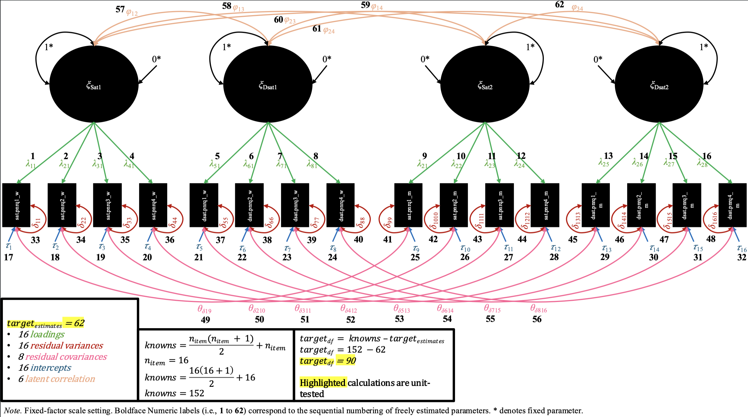
Counting # of parameters to be estimated, and degrees of freedom, for the configural invariance M-CDFM, with the pnrqM data

In the configural invariance M-CDFM, each partner shares the same number of factors, and the same general pattern of items loading onto factors, for which there are uniquely estimated loading values. Likewise, in the mean structure, each item has its own uniquely estimated intercept values. In the fixed-factor scaling of this model (shown in the path diagram), each factor has its latent variance constrained to 1 and its latent mean constrained to 0 for both partners (while all loadings and intercepts are estimated). In the marker-variable scaling (not shown in the diagram), the first loading of each factor is constrained to 1, and the intercept for the same item is constrained to 0, while the latent variance and mean are freely estimated.

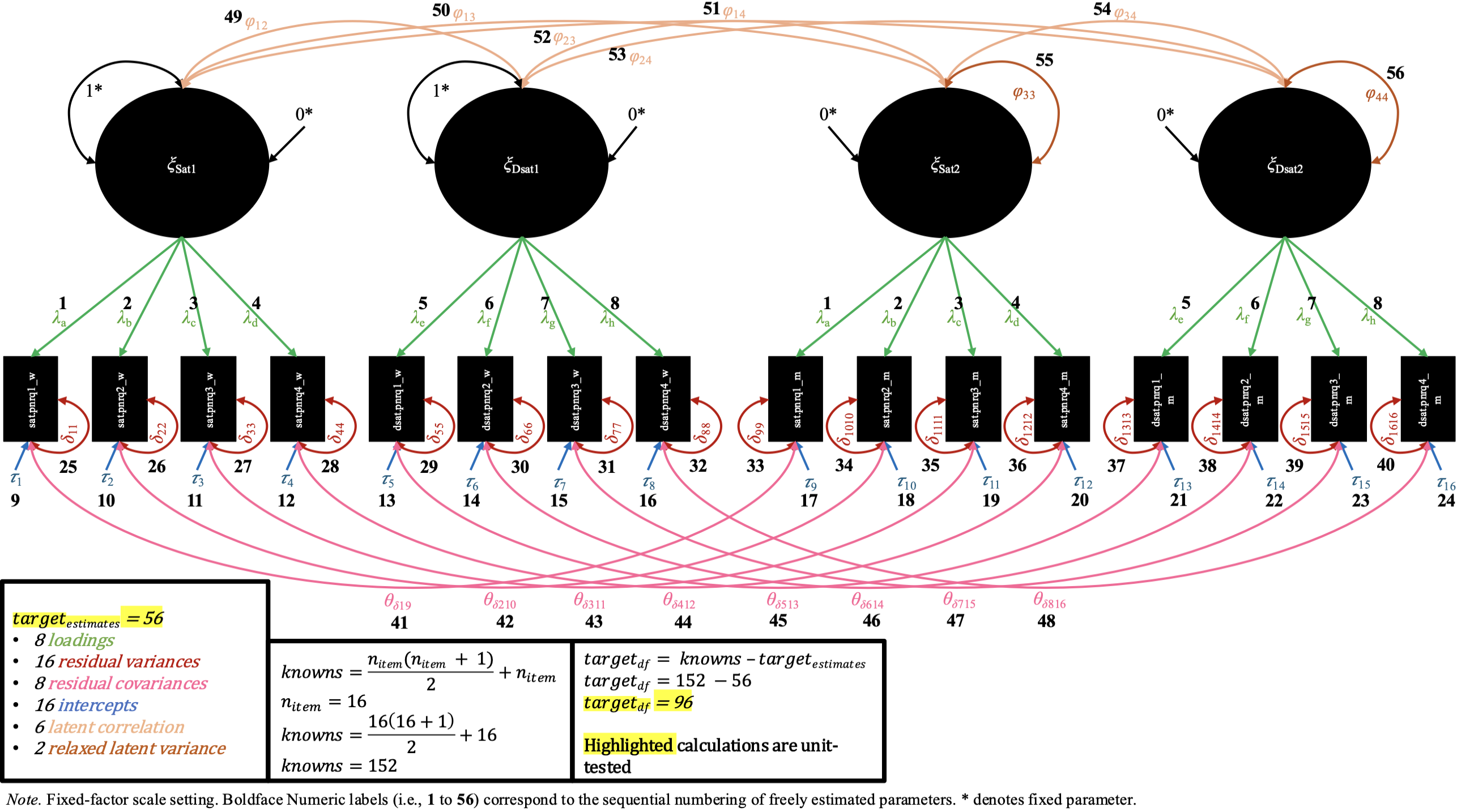
Counting # of parameters to be estimated, and degrees of freedom, for the loading invariance M-CDFM, with the pnrqM data

In the loading invariance M-CDFM, the loading values for the same items across partners are constrained to be equal. In the fixed-factor scaling, as a result of these constraints on the loadings, the constraints on the latent variances are not needed for both pairs of latent variances of each factor, and so we can freely estimate one of the latent variances for each factor (while the other remains constrained to 1). In the marker-variable scaling, the marker variable’s loading remains constrained to 1 for each pair of factors, while the other remaining loadings are constrained across partner.

Counting # of parameters to be estimated, and degrees of freedom, for the intercept invariance M-CDFM, with the pnrqM data

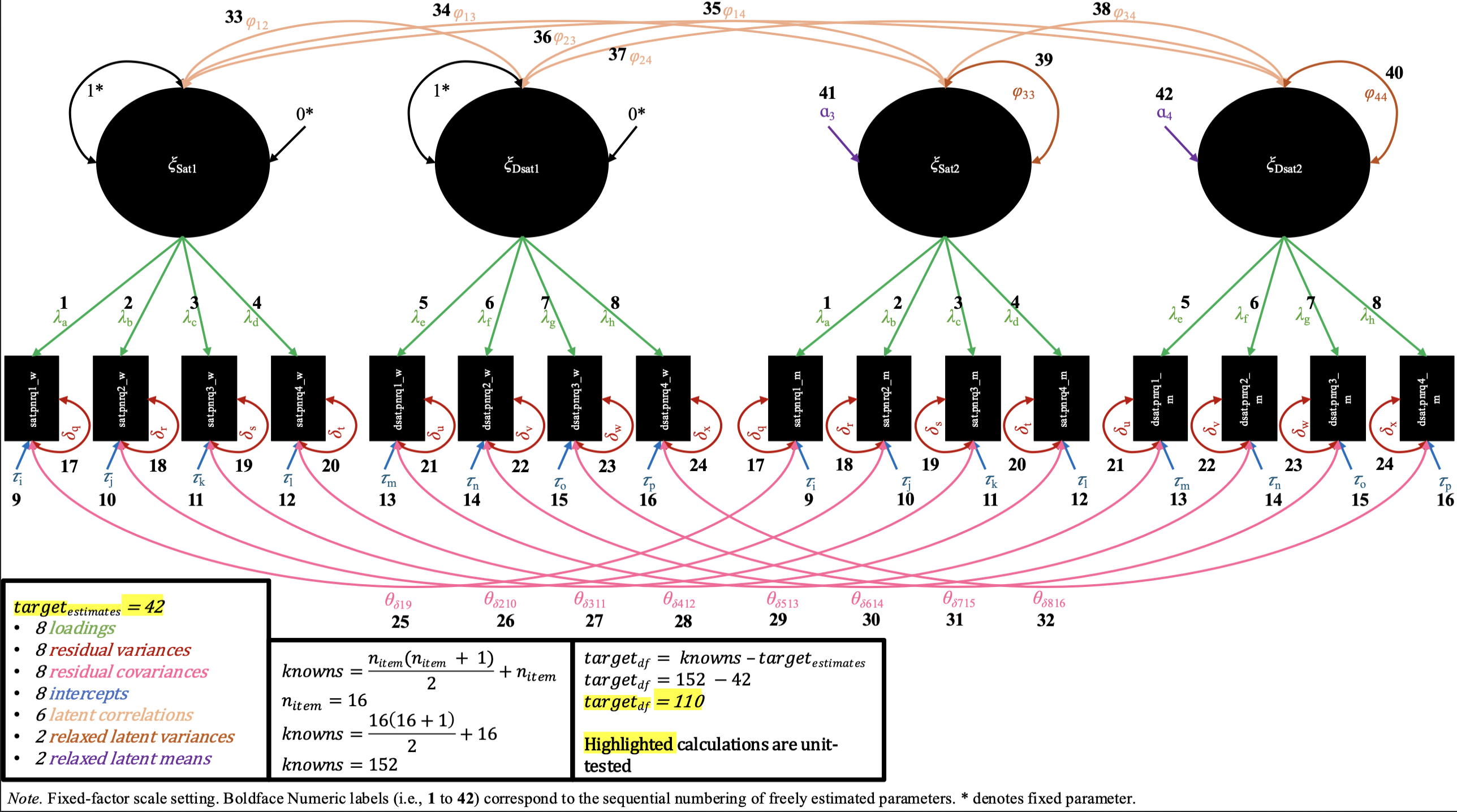
In the intercept invariance M-CDFM, the intercept values for the same items across partners are constrained to be equal. In the fixed-factor scaling, as a result of these constraints on the intercepts, the constraints on the latent means are not needed for both pairs of latent means of each factor, and so we can freely estimate one of the latent means for each factor (while the other remains constrained to 0). In the marker-variable scaling, the marker variable’s intercept remains constrained to 0 for each pair of factors, while the other remaining intercepts are constrained across partner.

Counting # of parameters to be estimated, and degrees of freedom, for the (less-frequently considered) residual invariance M-CDFM, with the pnrqM data

Finally, in the residual invariance M-CDFM, the residual variances for the same items across partners are constrained to be equal. The changes in syntax look identical for the fixed-factor and marker-variable scalings, as the constraints on the residual variances do not interact with the scale-setting choice a user makes (i.e., the residual variances are all uniquely estimated in configural, loading, and intercept invariance in both scalings, and therefore all pairs are available to be constrained across partner).

We hope these diagrams (and their corresponding tests) provide users a sense of comfort that the M-CDFM functionality in dySEM is working as intended, and that the model specifications it produces are correct.

QA Summary

Of course, we welcome any users alerting us of any errors in our model specifications (e.g., via GitHub issues on the dySEM GitHub Repo), and we will work to resolve any such errors as quickly as possible. Indeed, somewhat paradoxically, we feel the ability to publicly identify and fix errors is a strength of open-source software like dySEM: let us know what problems you find, and through code, we can fix them for everyone, forever, and for free!